本讲义基于 pandas 官方文档 10 Minutes to pandas 编写,结合中文读者习惯进行注释与讲解。
目录
对象创建
查看数据
选择数据
缺失值处理
运算
数据导入导出
索引
分组
连接
绘图
时间序列
Categorical
Plotting
Getting data in/out
导入 pandas 和 numpy
import pandas as pdimport numpy as np
对象创建
创建 Series
= pd.Series([1 , 3 , 5 , np.nan, 6 , 8 ])
0    1.0
1    3.0
2    5.0
3    NaN
4    6.0
5    8.0
dtype: float64
创建 DataFrame
= pd.date_range("20130101" , periods= 6 )
DatetimeIndex(['2013-01-01', '2013-01-02', '2013-01-03', '2013-01-04',
               '2013-01-05', '2013-01-06'],
              dtype='datetime64[ns]', freq='D')
= pd.DataFrame(np.random.randn(6 ,4 ), index= dates, columns= list ("ABCD" ))
2013-01-01
-0.520585
0.481536
-0.351331
-1.362496
2013-01-02
0.312901
1.507186
-0.652097
1.137791
2013-01-03
-0.873238
-1.893483
1.224852
-0.119387
2013-01-04
-0.488614
-0.179749
0.023712
1.182711
2013-01-05
0.237155
0.709768
-0.467694
-0.855296
2013-01-06
-0.257989
-1.401546
1.692584
-0.928318
由 dict 创建 DataFrame
= pd.DataFrame({"A" : 1. ,"B" : pd.Timestamp('20130102' ),"C" : pd.Series(1 , index= list (range (4 )), dtype= "float32" ),"D" : np.array([3 ] * 4 , dtype= "int32" ),"E" : pd.Categorical(["test" , "train" , "test" , "train" ]),"F" : "foo"
0
1.0
2013-01-02
1.0
3
test
foo
1
1.0
2013-01-02
1.0
3
train
foo
2
1.0
2013-01-02
1.0
3
test
foo
3
1.0
2013-01-02
1.0
3
train
foo
查看各列数据类型
A          float64
B    datetime64[s]
C          float32
D            int32
E         category
F           object
dtype: object
查看数据
查看头尾行
2013-01-01
-0.520585
0.481536
-0.351331
-1.362496
2013-01-02
0.312901
1.507186
-0.652097
1.137791
2013-01-03
-0.873238
-1.893483
1.224852
-0.119387
2013-01-04
-0.488614
-0.179749
0.023712
1.182711
2013-01-05
0.237155
0.709768
-0.467694
-0.855296
2013-01-04
-0.488614
-0.179749
0.023712
1.182711
2013-01-05
0.237155
0.709768
-0.467694
-0.855296
2013-01-06
-0.257989
-1.401546
1.692584
-0.928318
显示索引、列名和底层 numpy 数据
DatetimeIndex(['2013-01-01', '2013-01-02', '2013-01-03', '2013-01-04',
               '2013-01-05', '2013-01-06'],
              dtype='datetime64[ns]', freq='D')
Index(['A', 'B', 'C', 'D'], dtype='object')
array([[-0.52058527,  0.48153608, -0.35133101, -1.36249633],
       [ 0.31290141,  1.50718565, -0.65209664,  1.13779112],
       [-0.87323811, -1.8934827 ,  1.22485201, -0.11938684],
       [-0.48861365, -0.17974916,  0.02371156,  1.18271133],
       [ 0.23715514,  0.70976824, -0.46769407, -0.8552958 ],
       [-0.25798935, -1.40154591,  1.69258428, -0.92831789]])
描述性统计汇总
count
6.000000
6.000000
6.000000
6.000000
mean
-0.265062
-0.129381
0.245004
-0.157499
std
0.462917
1.302976
0.977027
1.096220
min
-0.873238
-1.893483
-0.652097
-1.362496
25%
-0.512592
-1.096097
-0.438603
-0.910062
50%
-0.373301
0.150893
-0.163810
-0.487341
75%
0.113369
0.652710
0.924567
0.823497
max
0.312901
1.507186
1.692584
1.182711
数据转置
A
-0.520585
0.312901
-0.873238
-0.488614
0.237155
-0.257989
B
0.481536
1.507186
-1.893483
-0.179749
0.709768
-1.401546
C
-0.351331
-0.652097
1.224852
0.023712
-0.467694
1.692584
D
-1.362496
1.137791
-0.119387
1.182711
-0.855296
-0.928318
按轴排序
= 1 , ascending= False )
2013-01-01
-1.362496
-0.351331
0.481536
-0.520585
2013-01-02
1.137791
-0.652097
1.507186
0.312901
2013-01-03
-0.119387
1.224852
-1.893483
-0.873238
2013-01-04
1.182711
0.023712
-0.179749
-0.488614
2013-01-05
-0.855296
-0.467694
0.709768
0.237155
2013-01-06
-0.928318
1.692584
-1.401546
-0.257989
2013-01-03
-0.873238
-1.893483
1.224852
-0.119387
2013-01-06
-0.257989
-1.401546
1.692584
-0.928318
2013-01-04
-0.488614
-0.179749
0.023712
1.182711
2013-01-01
-0.520585
0.481536
-0.351331
-1.362496
2013-01-05
0.237155
0.709768
-0.467694
-0.855296
2013-01-02
0.312901
1.507186
-0.652097
1.137791
选择数据
选择单列
2013-01-01   -0.520585
2013-01-02    0.312901
2013-01-03   -0.873238
2013-01-04   -0.488614
2013-01-05    0.237155
2013-01-06   -0.257989
Freq: D, Name: A, dtype: float64
通过切片选取多行(行标签)
2013-01-01
-0.520585
0.481536
-0.351331
-1.362496
2013-01-02
0.312901
1.507186
-0.652097
1.137791
2013-01-03
-0.873238
-1.893483
1.224852
-0.119387
"20130102" :"20130104" ]
2013-01-02
0.312901
1.507186
-0.652097
1.137791
2013-01-03
-0.873238
-1.893483
1.224852
-0.119387
2013-01-04
-0.488614
-0.179749
0.023712
1.182711
使用标签(loc)选择
A   -0.520585
B    0.481536
C   -0.351331
D   -1.362496
Name: 2013-01-01 00:00:00, dtype: float64
2013-01-01
-0.520585
0.481536
2013-01-02
0.312901
1.507186
2013-01-03
-0.873238
-1.893483
2013-01-04
-0.488614
-0.179749
2013-01-05
0.237155
0.709768
2013-01-06
-0.257989
-1.401546
"20130102" :"20130104" , ["A" , "B" ]]
2013-01-02
0.312901
1.507186
2013-01-03
-0.873238
-1.893483
2013-01-04
-0.488614
-0.179749
0 ], ["A" , "B" ]]
A   -0.520585
B    0.481536
Name: 2013-01-01 00:00:00, dtype: float64
按位置(iloc)选取
A   -0.488614
B   -0.179749
C    0.023712
D    1.182711
Name: 2013-01-04 00:00:00, dtype: float64
2013-01-04
-0.488614
-0.179749
2013-01-05
0.237155
0.709768
2013-01-02
0.312901
-0.652097
2013-01-03
-0.873238
1.224852
2013-01-05
0.237155
-0.467694
1 :3 , :]1 :3 ]
2013-01-01
0.481536
-0.351331
2013-01-02
1.507186
-0.652097
2013-01-03
-1.893483
1.224852
2013-01-04
-0.179749
0.023712
2013-01-05
0.709768
-0.467694
2013-01-06
-1.401546
1.692584
布尔索引
2013-01-02
0.312901
1.507186
-0.652097
1.137791
2013-01-05
0.237155
0.709768
-0.467694
-0.855296
2013-01-01
NaN
0.481536
NaN
NaN
2013-01-02
0.312901
1.507186
NaN
1.137791
2013-01-03
NaN
NaN
1.224852
NaN
2013-01-04
NaN
NaN
0.023712
1.182711
2013-01-05
0.237155
0.709768
NaN
NaN
2013-01-06
NaN
NaN
1.692584
NaN
= df.copy()"E" ] = ["one" , "one" , "two" , "three" , "four" , "three" ]
2013-01-01
-0.520585
0.481536
-0.351331
-1.362496
one
2013-01-02
0.312901
1.507186
-0.652097
1.137791
one
2013-01-03
-0.873238
-1.893483
1.224852
-0.119387
two
2013-01-04
-0.488614
-0.179749
0.023712
1.182711
three
2013-01-05
0.237155
0.709768
-0.467694
-0.855296
four
2013-01-06
-0.257989
-1.401546
1.692584
-0.928318
three
"E" ].isin(["two" , "four" ])]
2013-01-03
-0.873238
-1.893483
1.224852
-0.119387
two
2013-01-05
0.237155
0.709768
-0.467694
-0.855296
four
缺失值处理
pandas 使用 np.nan 代表缺失值。 可以用 dropna 删除含有缺失值的行,或者用 fillna 填充。
= df.reindex(index= dates[0 :4 ], columns= list (df.columns) + ["E" ])0 ]:dates[1 ], "E" ] = 1
2013-01-01
-0.520585
0.481536
-0.351331
-1.362496
1.0
2013-01-02
0.312901
1.507186
-0.652097
1.137791
1.0
2013-01-03
-0.873238
-1.893483
1.224852
-0.119387
NaN
2013-01-04
-0.488614
-0.179749
0.023712
1.182711
NaN
2013-01-01
-0.520585
0.481536
-0.351331
-1.362496
1.0
2013-01-02
0.312901
1.507186
-0.652097
1.137791
1.0
2013-01-01
-0.520585
0.481536
-0.351331
-1.362496
1.0
2013-01-02
0.312901
1.507186
-0.652097
1.137791
1.0
2013-01-03
-0.873238
-1.893483
1.224852
-0.119387
5.0
2013-01-04
-0.488614
-0.179749
0.023712
1.182711
5.0
2013-01-01
False
False
False
False
False
2013-01-02
False
False
False
False
False
2013-01-03
False
False
False
False
True
2013-01-04
False
False
False
False
True
运算
pandas 支持类似 numpy 的各类算术运算,且会自动对齐不同索引。
A   -0.265062
B   -0.129381
C    0.245004
D   -0.157499
dtype: float64
2013-01-01   -0.438219
2013-01-02    0.576445
2013-01-03   -0.415314
2013-01-04    0.134515
2013-01-05   -0.094017
2013-01-06   -0.223817
Freq: D, dtype: float64
= pd.Series([1 , 3 , 5 , np.nan, 6 , 8 ], index= dates).shift(2 )= "index" )
2013-01-01
NaN
NaN
NaN
NaN
2013-01-02
NaN
NaN
NaN
NaN
2013-01-03
-1.873238
-2.893483
0.224852
-1.119387
2013-01-04
-3.488614
-3.179749
-2.976288
-1.817289
2013-01-05
-4.762845
-4.290232
-5.467694
-5.855296
2013-01-06
NaN
NaN
NaN
NaN
Apply 方法
2013-01-01
-0.520585
0.481536
-0.351331
-1.362496
2013-01-02
-0.207684
1.988722
-1.003428
-0.224705
2013-01-03
-1.080922
0.095239
0.221424
-0.344092
2013-01-04
-1.569536
-0.084510
0.245136
0.838619
2013-01-05
-1.332380
0.625258
-0.222558
-0.016677
2013-01-06
-1.590370
-0.776288
1.470026
-0.944994
apply (lambda x: x.max () - x.min ())
A    1.186140
B    3.400668
C    2.344681
D    2.545208
dtype: float64
直方图统计
= pd.Series(np.random.randint(0 , 7 , size= 10 ))
6    5
5    2
3    1
1    1
4    1
Name: count, dtype: int64
字符串方法
= pd.Series(["A" , "B" , "C" , "Aaba" , "Baca" , np.nan, "CABA" , "dog" , "cat" ])str .lower()
0       a
1       b
2       c
3    aaba
4    baca
5     NaN
6    caba
7     dog
8     cat
dtype: object
合并
拼接
= pd.DataFrame(np.random.randn(10 , 4 ))= [df[:3 ], df[3 :7 ], df[7 :]]
0
0.149451
-1.716458
1.540956
-1.478438
1
-0.788580
0.942535
0.860695
1.277974
2
1.529843
0.978873
1.681723
0.128001
3
-1.031891
-0.645625
-0.101714
-0.894796
4
-1.341019
-0.400039
0.293592
-1.754958
5
-0.018467
-0.688119
0.063590
0.081667
6
0.042298
0.433534
0.509931
0.708851
7
0.631839
1.985047
0.612073
0.114068
8
1.433401
-0.619146
1.581860
-1.031054
9
1.029629
0.266897
-0.649012
0.456147
merge(类似 SQL join)
= pd.DataFrame({'key' : ['foo' , 'bar' ], 'lval' : [1 , 2 ]})= pd.DataFrame({'key' : ['foo' , 'bar' ], 'rval' : [4 , 5 ]})= 'key' )
分组 groupby
split-apply-combine
统计、聚合、转换
= pd.DataFrame({'A' : ['foo' , 'bar' , 'foo' , 'bar' , 'foo' , 'bar' , 'foo' , 'foo' ],'B' : ['one' , 'one' , 'two' , 'three' , 'two' , 'two' , 'one' , 'three' ],'C' : np.random.randn(8 ),'D' : np.random.randn(8 )'A' ).sum ()
A
bar
onethreetwo
-2.510037
1.483046
foo
onetwotwoonethree
2.931827
-2.711364
'A' , 'B' ]).sum ()
A
B
bar
one
-1.279562
-0.243084
three
-0.183928
-0.697683
two
-1.046547
2.423813
foo
one
1.735463
-3.088498
three
0.289137
0.215364
two
0.907227
0.161770
Reshaping
Stack/unstack
Pivot tables
= list (zip (* [['bar' , 'bar' , 'baz' , 'baz' ,'foo' , 'foo' , 'qux' , 'qux' ],'one' , 'two' , 'one' , 'two' ,'one' , 'two' , 'one' , 'two' ]]))= pd.MultiIndex.from_tuples(tuples, names= ['first' , 'second' ])= pd.DataFrame(np.random.randn(8 , 2 ), index= index, columns= ['A' , 'B' ])= df[:4 ]
first
second
bar
one
1.185040
0.718365
two
0.680732
0.058235
baz
one
1.726562
-0.828623
two
-0.362360
0.716046
= df2.stack()
first  second
bar    one     A    1.185040
               B    0.718365
       two     A    0.680732
               B    0.058235
baz    one     A    1.726562
               B   -0.828623
       two     A   -0.362360
               B    0.716046
dtype: float64
first
second
bar
one
1.185040
0.718365
two
0.680732
0.058235
baz
one
1.726562
-0.828623
two
-0.362360
0.716046
first
bar
A
1.185040
0.680732
B
0.718365
0.058235
baz
A
1.726562
-0.362360
B
-0.828623
0.716046
second
one
A
1.185040
1.726562
B
0.718365
-0.828623
two
A
0.680732
-0.362360
B
0.058235
0.716046
Pivot tables(透视表)
= pd.DataFrame({"A" : ["one" , "one" , "two" , "three" ] * 3 ,"B" : ["A" , "B" , "C" ] * 4 ,"C" : np.random.randn(12 ),"D" : np.random.randn(12 )= 'D' , index= ['A' , 'B' ], columns= ['C' ])
A
B
one
A
NaN
NaN
-0.374013
NaN
0.191885
NaN
NaN
NaN
NaN
NaN
NaN
NaN
B
NaN
NaN
NaN
NaN
NaN
NaN
-0.837664
NaN
NaN
NaN
-0.53223
NaN
C
0.069504
NaN
NaN
NaN
NaN
NaN
NaN
NaN
1.184217
NaN
NaN
NaN
three
A
NaN
NaN
NaN
NaN
NaN
NaN
NaN
NaN
NaN
0.025075
NaN
NaN
B
NaN
NaN
NaN
NaN
NaN
NaN
NaN
-0.050209
NaN
NaN
NaN
NaN
C
NaN
NaN
NaN
NaN
NaN
-0.813397
NaN
NaN
NaN
NaN
NaN
NaN
two
A
NaN
NaN
NaN
NaN
NaN
NaN
NaN
NaN
NaN
NaN
NaN
1.881732
B
NaN
-1.001614
NaN
NaN
NaN
NaN
NaN
NaN
NaN
NaN
NaN
NaN
C
NaN
NaN
NaN
-0.216438
NaN
NaN
NaN
NaN
NaN
NaN
NaN
NaN
时间序列
= pd.date_range('1/1/2012' , periods= 100 , freq= 'S' )= pd.Series(np.random.randint(0 , 500 , len (rng)), index= rng)'5Min' ).sum ()
C:\Users\Administrator\AppData\Local\Temp\ipykernel_56080\2503940574.py:1: FutureWarning: 'S' is deprecated and will be removed in a future version, please use 's' instead.
  rng = pd.date_range('1/1/2012', periods=100, freq='S')
2012-01-01    24577
Freq: 5min, dtype: int32
= pd.date_range('3/6/2012 00:00' , periods= 5 , freq= 'D' )= pd.Series(np.random.randn(len (rng)), rng)= ts.tz_localize('UTC' )
2012-03-06 00:00:00+00:00   -0.960792
2012-03-07 00:00:00+00:00   -2.119477
2012-03-08 00:00:00+00:00   -0.038033
2012-03-09 00:00:00+00:00   -0.125605
2012-03-10 00:00:00+00:00   -0.893517
Freq: D, dtype: float64
'US/Eastern' )
2012-03-05 19:00:00-05:00   -0.960792
2012-03-06 19:00:00-05:00   -2.119477
2012-03-07 19:00:00-05:00   -0.038033
2012-03-08 19:00:00-05:00   -0.125605
2012-03-09 19:00:00-05:00   -0.893517
Freq: D, dtype: float64
时间区间和频率转换
= pd.date_range('1/1/2012' , periods= 5 , freq= 'M' )= pd.Series(np.random.randn(len (rng)), index= rng)
C:\Users\Administrator\AppData\Local\Temp\ipykernel_56080\3446765465.py:1: FutureWarning: 'M' is deprecated and will be removed in a future version, please use 'ME' instead.
  rng = pd.date_range('1/1/2012', periods=5, freq='M')
2012-01-31   -0.054797
2012-02-29    1.442388
2012-03-31    0.846941
2012-04-30    0.750070
2012-05-31   -0.466189
Freq: ME, dtype: float64
2012-01   -0.054797
2012-02    1.442388
2012-03    0.846941
2012-04    0.750070
2012-05   -0.466189
Freq: M, dtype: float64
2012-01-01   -0.054797
2012-02-01    1.442388
2012-03-01    0.846941
2012-04-01    0.750070
2012-05-01   -0.466189
Freq: MS, dtype: float64
= pd.period_range('1990Q1' , '2000Q4' , freq= 'Q-NOV' )= pd.Series(np.random.randn(len (prng)), index= prng)
1990Q1   -0.275693
1990Q2   -1.237097
1990Q3    0.617560
1990Q4    1.263013
1991Q1   -1.938149
Freq: Q-NOV, dtype: float64
= ts.index.asfreq('M' , how= 'end' )
1990-02   -0.275693
1990-05   -1.237097
1990-08    0.617560
1990-11    1.263013
1991-02   -1.938149
Freq: M, dtype: float64
Categoricals
= pd.DataFrame({"id" : [1 , 2 , 3 , 4 , 5 , 6 ],"raw_grade" : ["a" , "b" , "b" , "a" , "a" , "e" ]})"grade" ] = df["raw_grade" ].astype("category" )"grade" ]
0    a
1    b
2    b
3    a
4    a
5    e
Name: grade, dtype: category
Categories (3, object): ['a', 'b', 'e']
"grade" ] = df["grade" ].cat.set_categories(["very good" , "good" , "very bad" ])"grade" ]
0    NaN
1    NaN
2    NaN
3    NaN
4    NaN
5    NaN
Name: grade, dtype: category
Categories (3, object): ['very good', 'good', 'very bad']
"grade" ] = df["grade" ].cat.set_categories(["very bad" , "bad" , "medium" , "good" , "very good" ])"grade" ]
0    NaN
1    NaN
2    NaN
3    NaN
4    NaN
5    NaN
Name: grade, dtype: category
Categories (5, object): ['very bad', 'bad', 'medium', 'good', 'very good']
= "grade" )
0
1
a
NaN
1
2
b
NaN
2
3
b
NaN
3
4
a
NaN
4
5
a
NaN
5
6
e
NaN
"grade" ).size()
C:\Users\Administrator\AppData\Local\Temp\ipykernel_56080\3951628473.py:1: FutureWarning: The default of observed=False is deprecated and will be changed to True in a future version of pandas. Pass observed=False to retain current behavior or observed=True to adopt the future default and silence this warning.
  df.groupby("grade").size()
grade
very bad     0
bad          0
medium       0
good         0
very good    0
dtype: int64
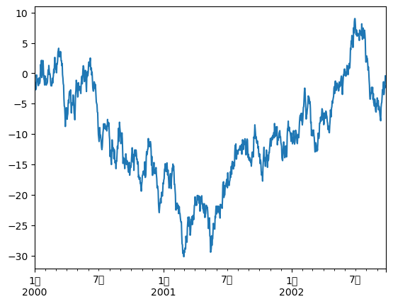
绘图
pandas 集成了 Matplotlib,可直接用 .plot() 快速画图。
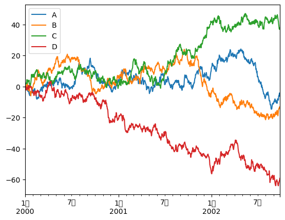
import matplotlib.pyplot as pltimport warningswith warnings.catch_warnings():"ignore" )= pd.Series(np.random.randn(1000 ), index= pd.date_range('1/1/2000' , periods= 1000 ))= ts.cumsum()
= pd.DataFrame(np.random.randn(1000 , 4 ), index= ts.index, columns= list ("ABCD" ))= df.cumsum()
c:\ProgramData\anaconda3\Lib\site-packages\IPython\core\pylabtools.py:170: UserWarning: Glyph 26376 (\N{CJK UNIFIED IDEOGRAPH-6708}) missing from font(s) DejaVu Sans.
  fig.canvas.print_figure(bytes_io, **kw)
c:\ProgramData\anaconda3\Lib\site-packages\IPython\core\pylabtools.py:170: UserWarning: Glyph 26376 (\N{CJK UNIFIED IDEOGRAPH-6708}) missing from font(s) DejaVu Sans.
  fig.canvas.print_figure(bytes_io, **kw)
数据读写
支持多种格式导入导出:CSV, HDF5, Excel, SQL, JSON 等
# 写入 CSV 'foo.csv' )# 读取 CSV 'foo.csv' ).head()
0
2000-01-01
-0.332295
0.167448
1.819971
0.262984
1
2000-01-02
-1.154339
-0.795782
1.476187
-0.507846
2
2000-01-03
-0.130460
0.149241
1.797390
0.417354
3
2000-01-04
-1.573087
0.423807
1.720803
-0.492286
4
2000-01-05
-1.842675
0.541527
1.728333
-1.907499
# 写入 Excel 'foo.xlsx' , sheet_name= 'Sheet1' )# 读取 Excel 'foo.xlsx' , 'Sheet1' ).head()
0
2000-01-01
-0.332295
0.167448
1.819971
0.262984
1
2000-01-02
-1.154339
-0.795782
1.476187
-0.507846
2
2000-01-03
-0.130460
0.149241
1.797390
0.417354
3
2000-01-04
-1.573087
0.423807
1.720803
-0.492286
4
2000-01-05
-1.842675
0.541527
1.728333
-1.907499